
When you’re working with a lot of data, it can be difficult to compare one or more rows with others that are towards the bottom of the workbook.
MS Excel freeze panes feature solves this problem by letting you lock specific rows so they’re always visible when you scroll. Here’s how to do that in Excel 2016.
There are two quick steps to freezing or locking rows.
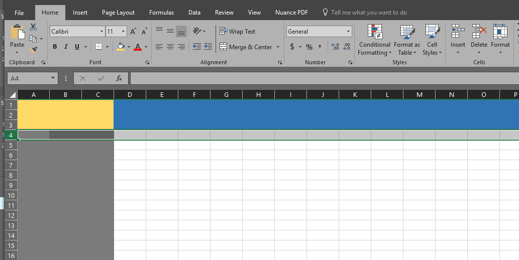
- Select the row right below the row or rows you want to freeze.
 (If you want to freeze columns, select the cell immediately to the right of the column you want to freeze).In this example, we want to freeze rows 1 to 3, so we’ve selected row 4.
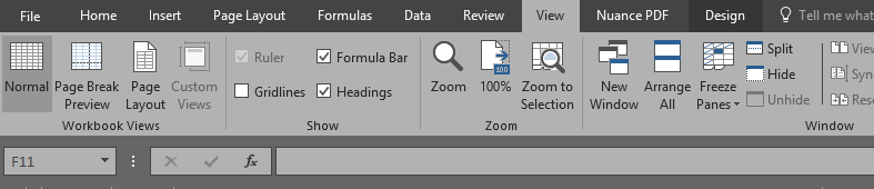
 - Go to the View tab
- Select the Freeze Panes command and choose “Freeze Panes.”
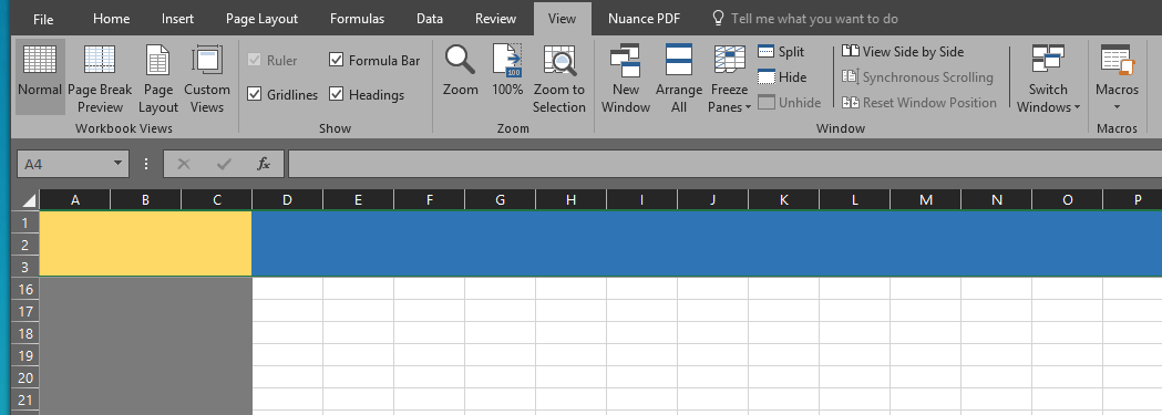
That’s all there is to it. As you can see in the image below, the frozen rows will stay visible when you scroll down.
Note: If you want to unfreeze the rows, go back to the Freeze Panes command and choose “Unfreeze Panes”.
Also note that under the Freeze Panes command, you can also choose “Freeze Top Row,” which will freeze the top row that’s visible (and any others above it) or “Freeze First Column,” which will keep the leftmost column visible when you scroll horizontally.
Also we can free both column and rows at the same time, for example if we want to freeze column (A, B, C) and rows (1, 2, 3), we can:
- Select cell immediate to the right of the column C (column D in this case) & below row 3 (row 4 in this case)
- Then to freeze it follow the same procedure, go to View tab, and select “Freeze Panes” drop-down, and select “Freeze Panes”.